9. Predictive analysis
Learning goals
By the end of this tutorial, you will be able to:
- Understand the difference between descriptive analysis and predictive analysis.
- Run a correlation test in R and interpret the result.
- Run a simple ANOVA and understand when to use post-hoc tests.
- Run a simple linear regression model in R.
- Apply these tools to a practice dataset involving COVID-19 cases and mobility.
Introduction to Predictive Analysis
Descriptive analysis helps us summarize what is happening in a dataset. Predictive analysis goes one step further by testing whether variables are statistically associated with one another.
In this tutorial, we introduce three common statistical tools:
- Correlation
- ANOVA
- Linear regression
These methods help us test relationships between variables and move beyond simple description.
This module is designed as a practical introduction. The goal is to help you understand when to use each test and how to interpret the results, rather than to cover all statistical details.
Required Packages
You only need to install packages once.
Part 1: Correlation
What is correlation?
A correlation test examines whether two numeric variables tend to move together.
- A positive correlation means that as one variable increases, the other also tends to increase.
- A negative correlation means that as one variable increases, the other tends to decrease.
- A correlation close to 0 suggests little or no linear relationship.
Here, we use the built-in mtcars dataset.
                   mpg cyl disp  hp drat    wt  qsec vs am gear carb
Mazda RX4         21.0   6  160 110 3.90 2.620 16.46  0  1    4    4
Mazda RX4 Wag     21.0   6  160 110 3.90 2.875 17.02  0  1    4    4
Datsun 710        22.8   4  108  93 3.85 2.320 18.61  1  1    4    1
Hornet 4 Drive    21.4   6  258 110 3.08 3.215 19.44  1  0    3    1
Hornet Sportabout 18.7   8  360 175 3.15 3.440 17.02  0  0    3    2
Valiant 18.1 6 225 105 2.76 3.460 20.22 1 0 3 1Step 1: Calculate a correlation
We test the relationship between car weight (wt) and horsepower (hp).
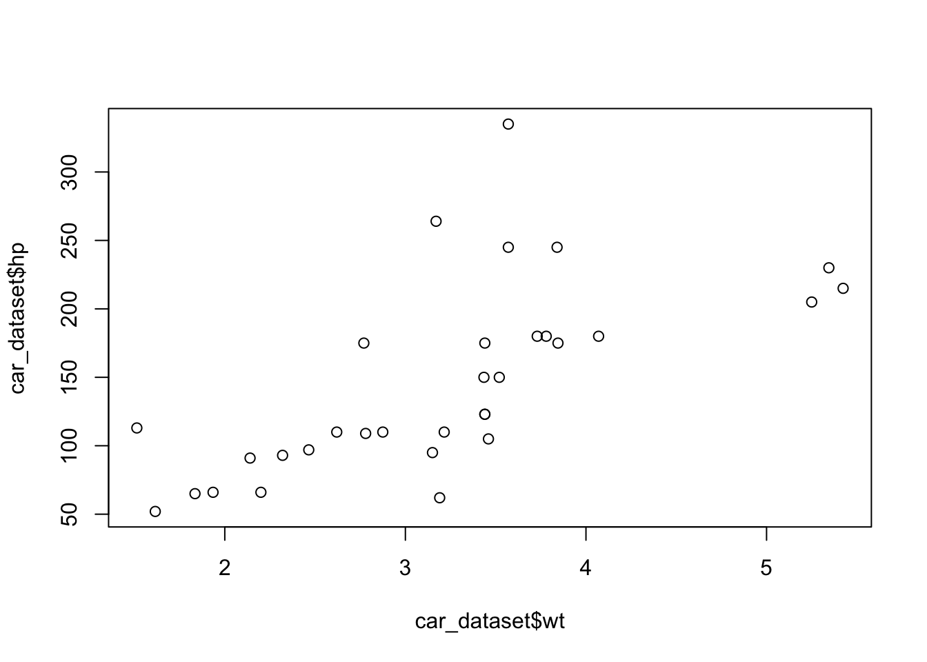
By default, cor() computes a Pearson correlation.
Step 2: Try a different correlation method
You can also use a different method, such as Spearman correlation.
Step 3: Report the p-value
If you need the test statistic and p-value, use cor.test().
    Pearson's product-moment correlation

data:  car_dataset$wt and car_dataset$hp
t = 4.7957, df = 30, p-value = 0.00004146
alternative hypothesis: true correlation is not equal to 0
95 percent confidence interval:
 0.4025113 0.8192573
sample estimates:
      cor
0.6587479 When reporting a correlation, it is useful to include:
- the correlation coefficient (
r) - the p-value
- a brief interpretation of the direction and strength of the relationship
Part 2: ANOVA
What is ANOVA?
ANOVA, or Analysis of Variance, is used when:
- the independent variable (IV) is categorical
- the dependent variable (DV) is numeric
Here, we test whether miles per gallon (mpg) differs across cars with different numbers of cylinders.
Step 1: Convert the IV to a factor
Step 2: Run ANOVA
Step 3: Run a post-hoc test
If the ANOVA result is statistically significant, a post-hoc test helps identify which groups differ from one another.
  Tukey multiple comparisons of means
    95% family-wise confidence level

Fit: aov(formula = mpg ~ cyl_factor, data = car_dataset)

$cyl_factor
          diff        lwr        upr     p adj
6-4  -6.920779 -10.769350 -3.0722086 0.0003424
8-4 -11.563636 -14.770779 -8.3564942 0.0000000
8-6 -4.642857 -8.327583 -0.9581313 0.0112287In ANOVA:
- the IV should be a factor
- the DV should be numeric
Part 3: Linear Regression
What is linear regression?
Linear regression estimates how much a numeric outcome changes as a predictor variable changes.
Here, we predict miles per gallon (mpg) using number of cylinders (cyl).
Step 1: Run a simple regression
Call:
lm(formula = mpg ~ cyl, data = car_dataset)

Residuals:
    Min      1Q  Median      3Q     Max
-4.9814 -2.1185  0.2217  1.0717  7.5186

Coefficients:
            Estimate Std. Error t value             Pr(>|t|)
(Intercept)  37.8846     2.0738   18.27 < 0.0000000000000002 ***
cyl          -2.8758     0.3224   -8.92       0.000000000611 ***
---
Signif. codes:  0 '***' 0.001 '**' 0.01 '*' 0.05 '.' 0.1 ' ' 1

Residual standard error: 3.206 on 30 degrees of freedom
Multiple R-squared:  0.7262,    Adjusted R-squared:  0.7171
F-statistic: 79.56 on 1 and 30 DF,  p-value: 0.0000000006113
You can also write the same model more compactly:
Call:
lm(formula = mpg ~ cyl, data = car_dataset)

Residuals:
    Min      1Q  Median      3Q     Max
-4.9814 -2.1185  0.2217  1.0717  7.5186

Coefficients:
            Estimate Std. Error t value             Pr(>|t|)
(Intercept)  37.8846     2.0738   18.27 < 0.0000000000000002 ***
cyl          -2.8758     0.3224   -8.92       0.000000000611 ***
---
Signif. codes:  0 '***' 0.001 '**' 0.01 '*' 0.05 '.' 0.1 ' ' 1

Residual standard error: 3.206 on 30 degrees of freedom
Multiple R-squared:  0.7262,    Adjusted R-squared:  0.7171
F-statistic: 79.56 on 1 and 30 DF,  p-value: 0.0000000006113
Step 2: Add another predictor
If you want to control for an additional variable, you can include multiple predictors in the same model.
Call:
lm(formula = mpg ~ cyl + wt, data = car_dataset)

Residuals:
    Min      1Q  Median      3Q     Max
-4.2893 -1.5512 -0.4684  1.5743  6.1004

Coefficients:
            Estimate Std. Error t value             Pr(>|t|)
(Intercept)  39.6863     1.7150  23.141 < 0.0000000000000002 ***
cyl          -1.5078     0.4147  -3.636             0.001064 **
wt           -3.1910     0.7569  -4.216             0.000222 ***
---
Signif. codes:  0 '***' 0.001 '**' 0.01 '*' 0.05 '.' 0.1 ' ' 1

Residual standard error: 2.568 on 29 degrees of freedom
Multiple R-squared:  0.8302,    Adjusted R-squared:  0.8185
F-statistic: 70.91 on 2 and 29 DF,  p-value: 0.000000000006809
Bonus: Display a model summary table
The modelsummary package provides a cleaner way to display regression results.
| (1) | |
|---|---|
| (Intercept) | 39.686 |
| (1.715) | |
| cyl | -1.508 |
| (0.415) | |
| wt | -3.191 |
| (0.757) | |
| Num.Obs. | 32 |
| R2 | 0.830 |
| R2 Adj. | 0.819 |
| AIC | 156.0 |
| BIC | 161.9 |
| Log.Lik. | -74.005 |
| F | 70.908 |
| RMSE | 2.44 |
Part 4: Practice Example with COVID-19 Cases and Mobility
In this example, we use the covidcases and mobility datasets from the HDSinRdata package.
# A tibble: 69,530 × 5
   state         county         week weekly_cases weekly_deaths
   <chr>         <chr>         <dbl>        <int>         <int>
 1 California    Marin             9            1             0
 2 California    Orange            9            3             0
 3 Florida       Manatee           9            1             0
 4 California    Napa              9            1             0
 5 New Hampshire Grafton           9            2             0
 6 Washington    Spokane           9            4             0
 7 California    San Francisco     9            3             0
 8 California    Placer            9            2             0
 9 Massachusetts Norfolk           9            1             0
10 Arizona       Maricopa          9            2             0
# ℹ 69,520 more rows# A tibble: 9,333 × 5
# Groups: state [51]
state date samples m50 m50_index
<chr> <chr> <int> <dbl> <dbl>
1 Alabama 2020-03-01 267652 10.9 76.9
2 Alabama 2020-03-02 287264 14.3 98.6
3 Alabama 2020-03-03 292018 14.2 98.2
4 Alabama 2020-03-04 298704 13.1 89.7
5 Alabama 2020-03-05 288218 14.8 102.
6 Alabama 2020-03-06 282982 17.9 126.
7 Alabama 2020-03-07 282326 16.3 114.
8 Alabama 2020-03-08 276150 10.9 77.0
9 Alabama 2020-03-09 290074 14.7 102.
10 Alabama 2020-03-10 286780 14.4 100.
# ℹ 9,323 more rowsStep 1: Prepare the dates
Before merging the datasets, we need to make sure the date formats are compatible.
Step 2: Merge the datasets
We merge the two datasets by state and date.
Step 3: Generate grouped summaries
This gives a quick overview of average mobility and total cases by state.
# A tibble: 51 × 4
   state       mean_m50 median_m50 cases_total
   <chr>          <dbl>      <dbl>       <int>
 1 Alabama         7.84       8.77      127616
 2 Alaska          2.12       2.45        6072
 3 Arizona         4.08       4.40      202373
 4 Arkansas        7.12       7.85       60600
 5 California      2.24       2.17      716585
 6 Colorado        5.12       5.83       58118
 7 Connecticut     3.07       2.93       52899
 8 Delaware        3.89       4.11       17246
 9 Florida         4.61       5.14      630002
10 Georgia         6.49       7.41      254062
# ℹ 41 more rows
Step 4: Filter to three states
For this example, we compare:
- California
- Florida
- Hawaii
Step 5: Check the data structure
To run ANOVA, the IV (state) should be a factor and the DV (m50) should be numeric.
gropd_df [3,569 × 9] (S3: grouped_df/tbl_df/tbl/data.frame)
 $ state        : chr [1:3569] "California" "California" "California" "California" ...
 $ date         : Date[1:3569], format: "2020-03-01" "2020-03-01" ...
 $ samples      : int [1:3569] 902406 902406 902406 902406 902406 902406 902406 902406 902406 902406 ...
 $ m50          : num [1:3569] 9.72 9.72 9.72 9.72 9.72 ...
 $ m50_index    : num [1:3569] 312 312 312 312 312 ...
 $ county       : chr [1:3569] "Marin" "Orange" "Napa" "San Francisco" ...
 $ week         : num [1:3569] 10 10 10 10 10 10 10 10 10 10 ...
 $ weekly_cases : int [1:3569] 1 2 0 14 4 5 2 1 1 23 ...
 $ weekly_deaths: int [1:3569] 0 0 0 0 0 1 0 0 0 0 ...
 - attr(*, "groups")= tibble [3 × 2] (S3: tbl_df/tbl/data.frame)
  ..$ state: chr [1:3] "California" "Florida" "Hawaii"
  ..$ .rows: list<int> [1:3]
  .. ..$ : int [1:1541] 1 2 3 4 5 6 7 8 9 10 ...
  .. ..$ : int [1:1770] 1542 1543 1544 1545 1546 1547 1548 1549 1550 1551 ...
  .. ..$ : int [1:258] 3312 3313 3314 3315 3316 3317 3318 3319 3320 3321 ...
  .. ..@ ptype: int(0)
..- attr(*, ".drop")= logi TRUEStep 6: Run ANOVA
Step 7: Run a post-hoc test
  Tukey multiple comparisons of means
    95% family-wise confidence level

Fit: aov(formula = m50 ~ state, data = filtered_data)

$state
                         diff        lwr       upr p adj
Florida-California  2.3782721  2.2237380  2.532806     0
Hawaii-California   0.7575374  0.4591798  1.055895     0
Hawaii-Florida     -1.6207347 -1.9163114 -1.325158     0
Checking assumptions before ANOVA
Technically, ANOVA assumes that group variances are reasonably equal. One common test is Levene’s test.
Levene's Test for Homogeneity of Variance (center = median)
        Df F value            Pr(>F)
group    2  27.054 0.000000000002182 ***
      3566
---
Signif. codes:  0 '***' 0.001 '**' 0.01 '*' 0.05 '.' 0.1 ' ' 1
If:
p > 0.05, the equal-variance assumption is metp < 0.05, the assumption is not met
If the assumption is not met, you can use Welch’s ANOVA instead.
Post-hoc comparison after Welch’s ANOVA
Here, we use pairwise t-tests with a Bonferroni correction.
    Pairwise comparisons using t tests with pooled SD

data:  filtered_data$m50 and filtered_data$state

        California           Florida
Florida < 0.0000000000000002 -
Hawaii  0.0000000087         < 0.0000000000000002

P value adjustment method: bonferroni You do not always need to run both standard ANOVA and Welch’s ANOVA in a final analysis. In teaching, however, comparing them can help students understand why assumptions matter.
Summary
In this chapter, you learned how to:
- calculate and interpret a correlation
- run ANOVA and post-hoc tests
- estimate a simple and multiple linear regression model
- merge and analyze real-world datasets in R
These methods are foundational for predictive analysis because they allow researchers to test whether variables are related in meaningful ways. In practice, choosing the right test depends on the type of variables you have and the research question you want to answer.